Using Pyslise

This document contains a few examples illustrating the usage of PySlise.

Mathieu problem

The Mathieu problem is given as: Find eigenfunctions \(\varphi\) and eigenvalue \(E\) for which

\[\frac{d^2}{dx^2}\varphi(x) + (E-2\cos(2x))\varphi(x) = 0\]

on \([0, \pi]\). The boundary conditions are: \(\varphi(0) = \varphi(\pi) = 0\).

This can be transformed to a Schrödinger equation with \(V(x) = 2\cos(2x)\). Solving this equation with PySlise is fairly easy:

from pyslise import Pyslise
from math import pi, cos

problem = Pyslise(lambda x: 2*cos(2*x), 0, pi, tolerance=1e-5)
left = (0, 1)
right = (0, 1)
eigenvalues = problem.eigenvaluesByIndex(0, 10, left, right)

The variable eigenvalues contains a list of tuples. Each tuple has as the first element the index of the eigenvalue and as second argument the eigenvalue itself. This example is a minimal example of how to use PySlise.

One could go further and ask for an estimation of the error for each eigenvalue. This data can be formatted in a nice table:

print('index  eigenvalue     error')
for index, E in eigenvalues:
    error = problem.eigenvalueError(E, left, right)
    print(f'{index:>5} {E:>11.5f} {error:>9.1e}')

index	eigenvalue	error
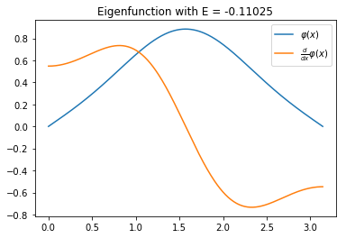
0	-0.11025	6.3e-08
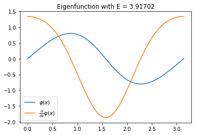
1	3.91702	1.2e-08
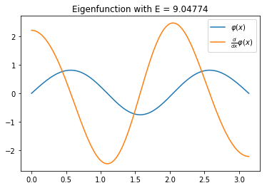
2	9.04774	2.9e-08
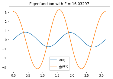
3	16.03297	2.6e-09
4	25.02084	1.3e-07
5	36.01429	6.5e-09
6	49.01042	1.2e-07
7	64.00794	5.0e-08
8	81.00625	4.5e-08
9	100.00505	2.4e-08

Depending on the version of PySlise or Python, or difference in hardware, your results may differ slightly.

Eigenfunctions

With matplotlib it is straightforward to make a plot of the eigenfunctions. The syntax is similar to MATLAB’s.

import numpy
import matplotlib.pyplot as plt

xs = numpy.linspace(0, pi, 300)
for index, E in eigenvalues:
    phi, d_phi = problem.eigenfunction(E, left, right, xs)

    plt.figure()
    plt.title(f'Eigenfunction with E = {E:.5f}')
    plt.plot(xs, phi, xs, d_phi)
    plt.legend(['$\\varphi(x)$', '$\\frac{d}{dx}\\varphi(x)$'])
    plt.show()

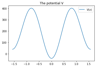
Coffey-Evans

The Coffey Evans problem is given by the potential:

\[V(x) = -2\beta\cos(2 x)+\beta^2\sin(2 x)^2\]

and the domain \([-\frac{\pi}{2}, \frac{\pi}{2}]\) with Dirichlet boundary conditions.

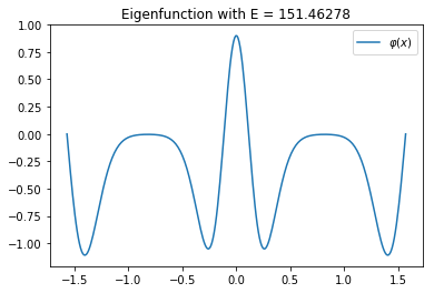
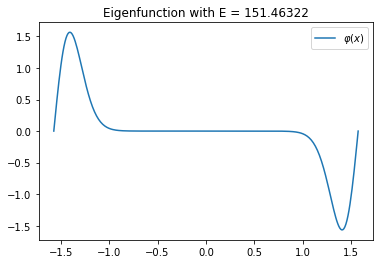
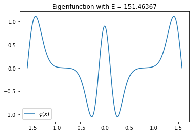
For rising \(\beta\), it is a well known hard problem, because there are triplets of close eigenvalues. On the other hand, the problem is symmetric and a few optimizations can be made. Pyslise implements this as PysliseHalf, indicating half range reduction is applied, because of the symmetry.

from pyslise import PysliseHalf
from math import pi, cos, sin

B = 20
problem = PysliseHalf(lambda x: -2*B*cos(2*x)+B**2*sin(2*x)**2,
                      pi/2, tolerance=1e-5)
side = (0, 1)
eigenvalues = problem.computeEigenvaluesByIndex(0, 10, side)
for i, E in eigenvalues:
    print(f'{i:3} {E:>10.6f}')

Index	Eigenvalue
0	-0.000000
1	77.916196
2	151.462778
3	151.463224
4	151.463669
5	220.154230
6	283.094815
7	283.250744
8	283.408735
9	339.370666

Adapting the code for plotting, the first triplet of close eigenvalues can be visualized. For completeness, also the potential itself is plotted.

import numpy
import matplotlib.pyplot as plt

xs = numpy.linspace(-pi/2, pi/2, 300)

plt.figure()
plt.title(f'The potential V')
plt.plot(xs, list(map(V, xs)))
plt.legend(['$V(x)$'])
plt.show()

for index, E in eigenvalues:
    phi, d_phi = problem.computeEigenfunction(E, side, xs)

    plt.figure()
    plt.title(f'Eigenfunction with E = {E:.5f}')
    plt.plot(xs, phi)
    plt.legend(['$\\varphi(x)$'])
    plt.show()